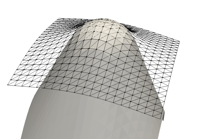
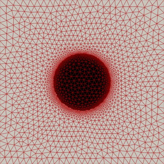
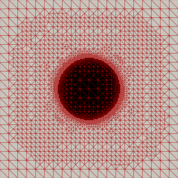
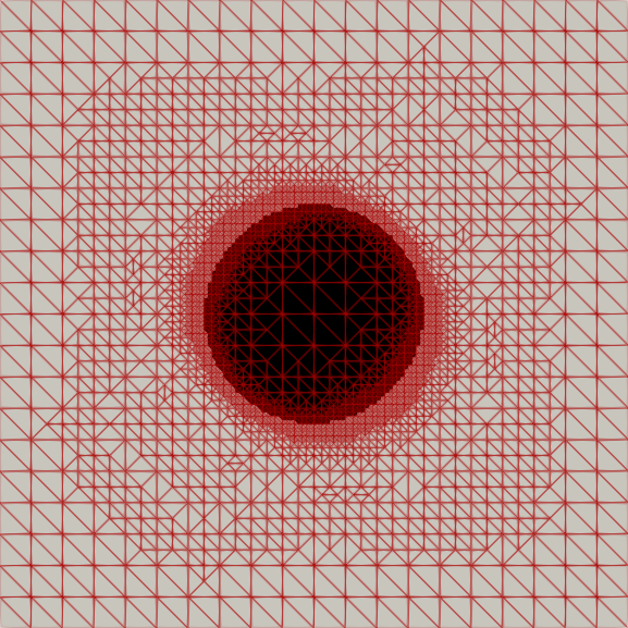
Adaptive Mesh Refinement for Variational Inequalities
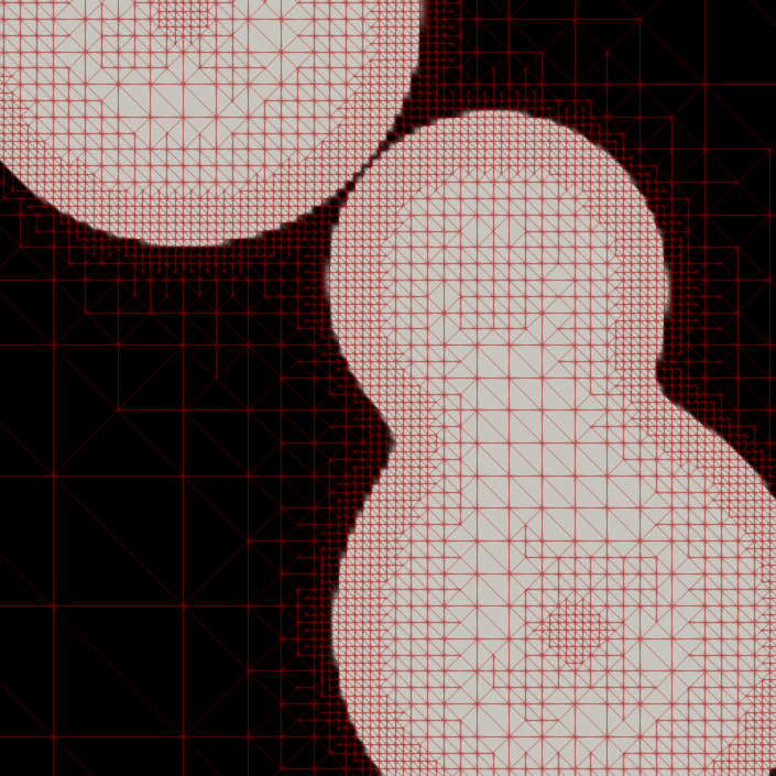
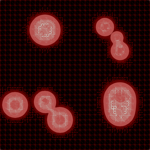
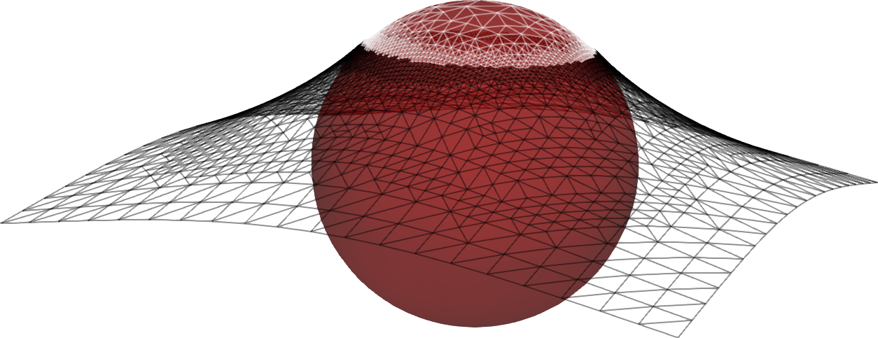
My master’s research centered on free-boundary problems, like the obstacle problem, which appear in many scientific and engineering applications. I developed and implemented several new parallel adaptive mesh refinement strategies to accurately localize the free boundary in the finite element solution of these problems. The methods were implemented using the Firedrake FE library and applied to both classical Laplacian obstacle problems and a shallow ice flow problem for predicting glaciation. You can find a detailed explanation in the paper and the source code in the project repository.
Graph Cut Image Segmentation
Throughout my master’s degree, I focused on projects at the intersection of graph theory and numerical methods. During my time at the Museum of the North Herbarium lab and the Cold Regions Research and Engineering Laboratory, I primarily worked on computer vision methods, including segmentation, object detection, clustering, and landmark detection.
To unify the concepts I learned in my graduate graph theory course, I presented several formulations of graph flow problems as linear programming problems, along with the theory behind the network simplex method. These methods intersect interestingly in applications like graph cut image segmentation. Below is a demonstration I created for the class, implementing the techniques described in Li et al. (2004).
Leaf Segmentation Tool
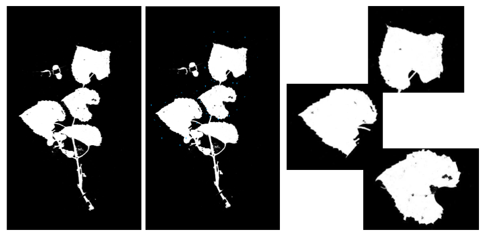
This script is essentially a polygonal cropping tool, but was made to facilitate the preprocessing step of herbarium sheets as outlined during the presentation at Botony 2022. The script begins by prompting the user for their images directory, then the first image is displayed. The user selects a bounding box with the cursor and the space button is used to crop. Pressing the escape key proceeds to the next image where the user can again crop as desired. Below is an example of how the script displays and image, the user then selects bounding boxes in cyan, and the resultant leaf level masks. This tool and further documentation can be found here.
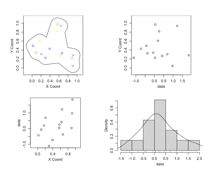
Custom Borders for ‘geoR’ Package Objects.
The following get_borders(my.lonlat, concavity_param, frac) function finds the concave hull of your geoR data object, and generates a nice bounding border for your geoR object.
The function takes three parameters, my.lonlat, concavity_param, and frac. The my.lonlat parameter is simply a 2 column matrix of your lon,lat data. The concavity_param argument is a relative measure of concavity. When set to 1 we get a concave hull, for sufficiently large concavity_param we get the convex hull. The frac argument extends the border in every direction. The function uses the geoR, concaveman, and rgeos packages. The following is an example, and results.
install.packages(c("geoR", "concaveman", "rgeos"))
library(geoR)
library(concaveman)
library(rgeos)

source("get_borders.r") # or copy and paste directly into RStudio

## Generating Data
set.seed(5834)
n <- 14
lons <- runif(n)
lats <- runif(n)
yyy <- rnorm(n)
## Creating geoR object
mygeo <- as.geodata(cbind(lons,lats,yyy))
## Custom Border
mygeo$borders <- get.borders(cbind(lons,lats), concavity_param = 1, frac = .15)

## Plotting
plot(mygeo)